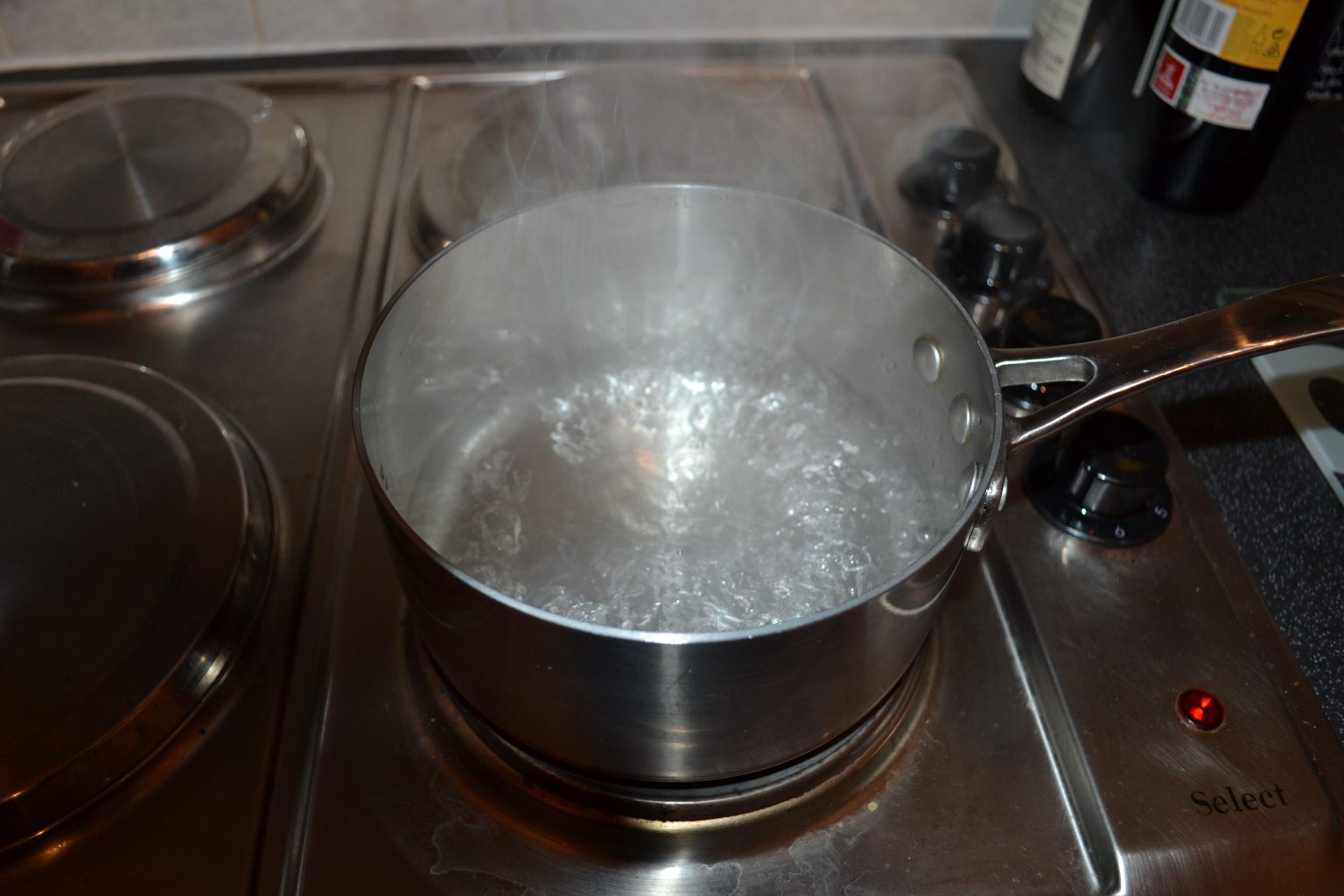
Multiphase flows are everywhere, one example is in boiling
fluids
(a two-phase gas-liquid flow).
Steam is used to transfer heat in nearly every
industry, and it needs boilers to “raise” it.
For forced boiling, we require two-phase corrections
for the heat transfer coefficients. \begin{align*} h_{cb} =
f_c h_{conv.} + f_s h_{nb} \end{align*}
In the simplest models, we needed to consider the
dimensionless parameter known as the
Lockhart-Martinelli parameter, $X_{tt}$, to
calculate these corrections ($f_c$ and $f_s$).
This parameter is part of the foundation of simple
multiphase flow pressure drop calculations.
Modern methods for estimating multiphase flow properties
are "mechanistic" and are moving beyond this parameter;
however, many correlations for other properties (such as
heat transfer) have yet to catch up so we cover it here.
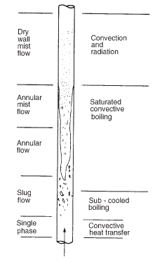
Forced boiling in a vertical tube.
Multiphase flow is a key challenge in oil and gas production
and its this industry that has driven the development of
mechanistic flow models.
The fluid coming out of oil wells and passing through rigs and
pipelines are a mixture of gas, oil, water, other chemicals, and
solids from formation erosion.
This multi-phase mixture is piped to shore in huge (100's km)
pipelines, to be treated at an onshore oil/gas plant.
Over a long enough pipeline, any multiphase flow will go
to
slug flow.
Taken from http://www.wlv.com/products/databook
When these “slugs” of liquid arrive at the oil and gas
terminal/plant, they can be enormous and need to be “caught” to
prevent them overwhelming the plant equipment.
Installation of a slugcatcher in Ireland. These pieces of
equipment exist to prevent slugs overwhelming the plant and to
separate the gas and liquid phases. Multiple pipes are used to
expand the flow as they are the cheapest way to construct the
large volumes needed to decellerate and settle out the flow.
Slug flow is always problematic as it is unsteady-state,
oscillatory or intermittent flow, which is hard to design for.
With a long oil and gas pipeline we cannot always avoid
slug flow, but in smaller process equipment we might avoid it in
design, if we can predict the
flow pattern!
In the oil and gas industry, the mechanistic models of
olga and
LedaFlow are used to perform these complex calculations
for long pipelines. Mechanistic models attempt to classify the
type of flow, and apply particular models depending on the
flow pattern.
Initially, flow pattern maps were used to predict the
flow pattern. Now, the flow pattern is more a statement of
which mechanistic model we have will have the best
predictions based on experimental data.
In multiphase flow in horizontal pipes, a common set
of flow regimes are identified to the right.
Originally, these patterns were identified by eye, or by
some measurement of the pressure fluctuations. Now,
empirical evidence of which model best fits a mechanistic
model is used to select the flow pattern (i.e. laminar
stratified flow is well approximated by the model in the
tutorials, thus any flow well approximated by that model is
"defined" as stratified flow).
Visual/pressure fluctuation identification is problematic
as there are no hard and fast definitions, and many flow types
blend from one to another… Bubble $\to$ Plug $\to$ Slug
$\to$ Wavy $\to$ Stratified or Annular $\to$ Spray.
Horizontal two-phase flow patterns, taken from
Coulson and Richardson Vol. 1.
Bubble, Plug and Slug flow are examples of
Intermittent
flow.
This is because in these regions the flow of gas or liquid
has strong fluctuations in the pressure or flow velocities
of the individual phases.
Obviously this regime of flow is difficult to design
with as there is no static equilibrium, and fluctuations must
be accommodated for (e.g., the slug catchers)
The “slugs” can even be dangerous, especially when
they “impact” upon bends or obstacles in the flow.
It is often desirable to aim for annular flow over the
range of expected flow rates in the pipe.
Horizontal two-phase flow patterns.
Without using mechanistic models, the simplest way to
estimate the flow pattern in a pipe is using a
flow pattern map.
There are hundreds of these maps in existence, some
generalised to arbitrary fluids but most are for air/water
mixtures and are not very general (this is why mechanistic
models are being developed).
The axis of these graphs are usually functions of the
liquid (y-axis) and the gas (x-axis) flow rate.
The most axes are the
superficial
velocities
\begin{align*}
u_L &= \frac{\dot{V}_{Liq.}}{A} &
u_G &= \frac{\dot{V}_{Gas}}{A}
\end{align*}
These are the velocities of each phase, calculated as
if they were flowing alone in the pipe.
Horizontal two-phase flow patterns.
Chhabra-Richardson flow map for flow in Horizontal
Pipes. Most maps are constructed using air-water flows at
atmospheric pressure and temperature thus they must be used
with caution for other flows.
The Chharbra-Richardson flow map is popular as it can be
used for a wide range of pipes and corrections for the
effect of different fluid properties seems to be smaller
than most.
The graph even appears to work well for gas and shear
thinning suspensions mixtures.
There is even suggestion that the map can be used for
vertical flow according to C&R vol 1, but research in
general has moved away from graphical flow maps.
Chhabra-Richardson flow map for flow in Horizontal Pipes.
In vertical flow, the principle flow patterns are much
simpler. This is because gravity does not cause an
asymmetric separation.
Also, the dangers of intermittent flow are not as
severe, although oscillations can still occur.
The intermittent flow patterns are the slug and churn
flow.
Often, an annular flow pattern is desirable in
vertical flow as it minimises the pressure drop:
Vertical two-phase flow patterns.
In vertical flows, the flow pattern maps are usually
expressed in terms of the mass flux (kg m${}^{-2}$s${}^{-1}$).
\begin{align*}
G_L &= \frac{\rho_L \dot{V}_{Liq.}}{A} = \rho_L u_L \\ G_G
&= \frac{\rho_G \dot{V}_{Gas}}{A} = \rho_G u_G
\end{align*}
and the total mass flux is
$G=G_L+G_G$.
The terms used in a popular vertical flow map,
the Hewitt-Roberts map, are the momentum fluxes
\begin{align*}
\frac{G_L^2}{\rho_L} &= \rho_L u_L^2 & \frac{G_G^2}{\rho_G}
&= \rho_G u_G^2
\end{align*}
Vertical two-phase flow patterns.
Vertical boiling is one of many cases of multiphase
flow, where every vertical flow pattern can be observed.
Another case might be bubbles coalescing as they rise
up a pipe (E.g., in a gas lift pump, see C&R, Vol.1,
Sec. 8.4.1).
Forced boiling in a vertical tube.
Turbulence is tricky in multiphase flows as each phase
individually may be laminar or turbulent.
We then have to calculate a Reynolds number for each phase,
but using generalised Reynolds numbers such as the
Metzner-Reed definition requires solutions for the flow,
which is difficult in any complex flow.
A simple definition arises from using the superficial
velocities \begin{align*} \text{Re}_L &=
\frac{\rho_L u_L D}{\mu_L} = \frac{G_L D}{\mu_L} &
\text{Re}_G &= \frac{\rho_G u_G D}{\mu_G} =
\frac{G_G D}{\mu_G} \end{align*} in the standard Reynolds
number definition.
The actual flow velocities will be higher than the
superficial velocities as the other phase occupies some of the
pipe.
As a result, the critical Reynolds number appears to be
somewhere in the range of $1000\lesssim
\text{Re}_{crit}\lesssim 2000$.
If we want to calculate the pressure drop in a multi-phase
liquid, there are only a few times we might be able to do this
analytically.
One example is the
Stratified flow studied in the tutorials.
This would form part of a mechanistic model and would be used
for any flows which approach laminar stratified flow.
Another complication of multiphase flow arises from the
expansion of the gas phase. As the pressure drops, the gas
expands, which causes the gas velocity to increase and this
ends up accelerating the liquid phase.
We will need to use empirical expressions to capture this
frictional pressure drop, and equations of state to capture
the expansion effects (compressible flow)... hence why
simulation is popular.
In this course we will use some simpler and older expressions
for predicting pressure drop. These empirical multiphase
correlations are often expressed in terms of the
Lockhart-Martinelli parameter.
\begin{align*}
X^2 =
\frac{\left(\Delta p/L\right)_{liq.-only}}{\left(\Delta
p/L\right)_{gas-only}}
\end{align*}
This parameter is the ratio of the theoretical pressure
drops if each phase, with the same mass flow rate, was flowing
through the pipe on its own.
We calculate these pressure drops in the standard way,
for each phase
in pipes:
Calculate the Reynolds number.
Select the expression for the friction factor $C_f$.
\begin{align*}
C_f&=16/Re & C_f&=0.079 \text{Re}^{-1/4}
\end{align*}
Use it in the Darcy-Wiesbach expression.
\begin{align*}
\frac{\Delta p}{L} = \frac{C_f \rho\left\langle v\right\rangle^2}{R}
\end{align*}
Once this is done for both phases, you can calculate the
Lockhart-Martinelli parameter!
One of the simplest multiphase pressure drop calculations
uses
multiphase multipliers
which allow the calculation of the two phase pressure drop.
\begin{align*}
\Delta p_{two-phase} = \Phi^2_{liq.} \Delta p_{liq.-only} = \Phi^2_{gas} \Delta p_{gas-only}
\end{align*}
The two phase multiplier $\Phi^2$
is calculated from
semi-empirical expressions, such as
Chisholm's relation,
which take into account frictional pressure drop:
\begin{align*}
\Phi^2_{gas} &= 1 + c X + X^2 &\\
\Phi^2_{liq.} &= 1 + \frac{c}{X}+\frac{1}{X^2} &
c &= \begin{cases}
20& \text{turbulent liquid & turbulent gas}\\
12& \text{laminar liquid & turbulent gas}\\
10& \text{turbulent liquid & laminar gas}\\
5& \text{laminar liquid & laminar gas}
\end{cases}
\end{align*}
We can now calculate expressions for the pressure drop in
two-phase flow. The full procedure is
Calculate the Reynolds number for each phase.
Calculate the single-phase pressure drops$\Delta
p_{liq.-only}$
and
$\Delta p_{gas-only}$.
Use Chisholm's relation to calculate either$\Phi^2_{liq.}$
or
$\Phi^2_{gas}$.
Calculate the two-phase pressure drop!
We've found that we can calculate the
frictional
pressure drop
using the Lockhart-Martinelli parameter to work
out a two phase multiplier:
\begin{align*}
\Delta p_{two-phase} = \Phi^2_{liq.} \Delta p_{liq.-only} = \Phi^2_{gas} \Delta p_{gas-only}
\end{align*}
Friction is not the only mechanism by which pressure
energy may be lost. Another is through changes in the
hydrostatic head.
\begin{align*}
\Delta p_{two-phase} = \Phi^2_{liq.} \Delta p_{liq.-only} +
\rho_{two-phase} g \Delta Y
\end{align*}
In vertical flows the hydrostatic pressure drop can be the
dominant contribution to the pressure drop.
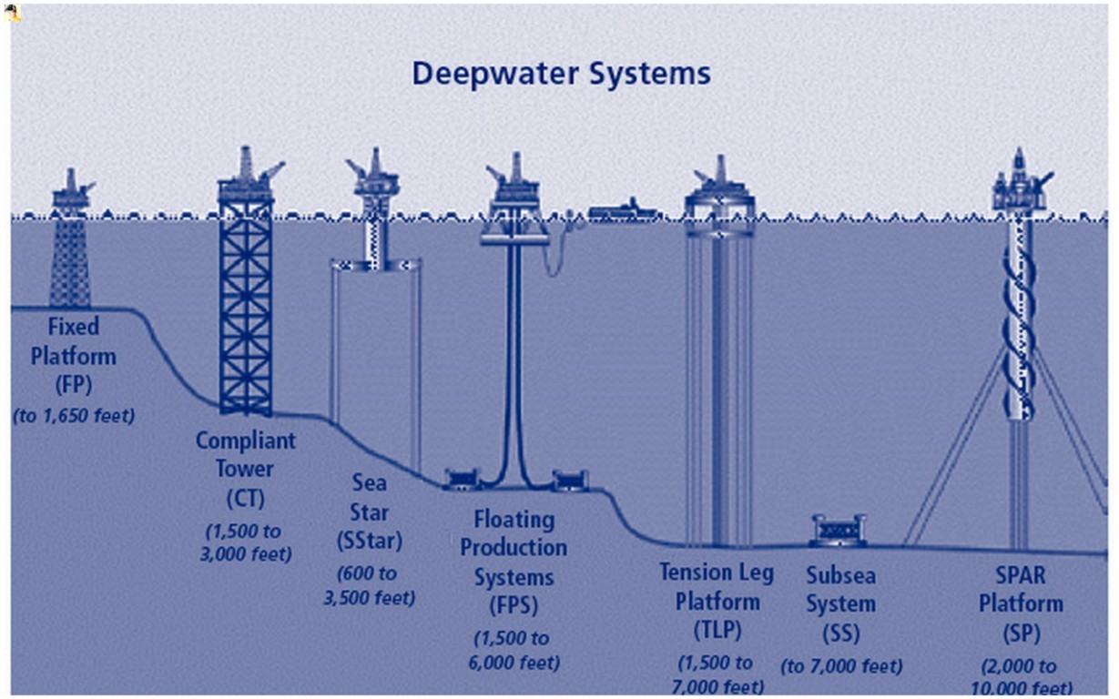
In the offshore industry there can be a lot of height for
the multiphase well fluid to travel, even once it is out of the
ground…
Offshore platform depths.
To calculate the hydrostatic pressure loss
$\rho_{two-phase} g \Delta Y$, we need the two-phase fluid
density.
If we knew the fraction of the pipe volume which is
occupied with liquid, $h$, we could easily calculate the
multiphase density like so
\begin{align*}
\rho_{two-phase} = h \rho_L + (1-h) \rho_G
\end{align*}
The parameter is a $h$
as it is known as the
liquid
hold-up.
$h$, in segregated flow between plates, is proportional to
the height of occupied by the liquid (Fluid 2) phase:
This value can literally be worth millions when trying to
estimate the contents/inventory and performance of a long offshore
pipeline.
The simplest estimate we can come up with for the liquid
hold-up is the
no-slip
estimate.
We assume that the liquid and gas phases are stuck
together, so that the volumes occupied in the pipe are
proportional to the volumetric flowrates!
\begin{align*}
h = \dot{V}_L / \left(\dot{V}_L + \dot{V}_G\right)
\end{align*}
This is not realistic as the gas phase usually
bypasses the liquid phase in segregated flows (but this
is not a bad approach for bubble or plug flows!).
For example, consider the two-phase laminar plate flow in
the tutorials:
\begin{multline*}
\frac{\dot{V}_1}{\dot{V}_2} = -
\frac{3\mu_2}{\mu_1}\frac{H^3}{h^3}
\left[(1+A_1)\left(1-\frac{h}{H}\right)
-\frac{A_1}{2}\left(1-\frac{h^2}{H^2}\right)
-\frac{1}{3}\left(1-\frac{h^3}{H^3}\right)
\right]
\times
\left[1+A_1\frac{3}{2}\frac{H}{h}\right]^{-1}
\end{multline*}
All the usual caveats of empirical expressions apply to
the expressions given for the liquid hold-up.
There is no one-size fits all expression, experimental
data is often needed or specialist simulation packages like
Olga
or
LedaFlow
are used.
However, C&R Vol.1, pg. 186 provides us with one
expression to use by Farooqi and Richardson for co-current flows
of Newtonian fluids and air in horizontal pipes.
\begin{align*}
h &=
\begin{cases}
0.186+0.0191 X & 1 < X < 5\\
0.143 X^{0.42} & 5 < X < 50\\
1/\left(0.97 + 19/X\right) & 50 < X < 500
\end{cases}
\end{align*}
This allows the calculation of the two-phase density and
then the hydrostatic pressure loss which can then be added to the
frictional pressure drop.
\begin{align*}
\Delta p_{two-phase} = \rho_{two-phase} g \Delta Y +
\Phi^2_{liq.} \Delta p_{liq.-only}
\end{align*}
It should now be obvious why annular flow is desirable in
many cases as it yields the lowest pressure drop in vertical flow.
The liquid hold-up is at a minimum and so is the density
which gives the minimum hydrostatic pressure loss.
The liquid hold-up is also proportional to the cross
sectional area of the pipe occupied by fluid.
The area which is available for liquid flow is
$A_{L}=h A$, and for gas flow is
$A_{G}=(1-h) A$.
We can use the no-slip hold-up to calculate
no-slip
velocities
or the actual hold-up to calculate
actual-velocities.
\begin{align*}
v_{L,no-slip} &= \dot{V}_L / (A h_{no-slip}) & v_{L,actual} &= \dot{V}_L / (A h_{actual})
\end{align*}
These improved estimates could be used to enforce a
maximum flow velocity to prevent wear/erosion or impact damage
etc.
One last, important consideration is that the gas in
multi-phase flow is
compressible.
As the pressure drops the gas flow expands, causing
the gas phase to accelerate. This implies that the flow pattern,
liquid hold up, and pressure drop will all change along the pipe.
We must be careful to consider compressible flow and
re-evaluate our pressure drop predictions along the length of the
pipe to compensate.
Analytical compressible flow is covered in detail in a
later course; however, you could always use finite difference
approaches to solve it!
Learning objectives
Flow pattern maps, which patterns there are an which ones
are intermittent and which are desirable.
The Reynolds number is calculated for each phase
separately using the superficial velocity, and the turbulent
transition is around $1000\to2000$.
We can calculate the Lockhart-Martinelli parameter and use
it to calculate a multiphase multiplier to work out the
frictional/accelerational pressure drop using emprircal
correlations.
The importance of the liquid hold up, the no-slip hold up
and the corresponding velocities.
The calculation of the multiphase density and the
hydrostatic pressure drop.