CADR Meeting: Particle Dynamics

Marcus N. Bannerman
[email protected]

Particle dynamics

• Particle dynamics is a single technique which can simulate all of the classical scales of dynamics.
• Here, the focus is molecular and granular systems, but the underlying technique is identical at all scales above.

Each of the $N$ particles represents some portion of the system's mass.

The motion of each particle is described by Newton's law:

As analytical solutions are not usually available for $N>2$ systems
(it will be demonstrated that they are available for some forces)
numerical integration is often used.

In granular (dissipative) systems, standard explicit techniques such as Runge-Kutta (i.e., ode45) and Gear's predictor-corrector (i.e. ode15s) are used.

In molecular (elastic) systems, they are much more picky. Only Symplectic (phase volume conserving) techniques are used.

Consider the simplest particle system, the spring-mass system.

Its exact solution is well known. For $r(t=0)=1$ and $v(t=0)=0$, we have:

\begin{align*} r(t) &= \cos(\omega\,t) & v(t) &= \sin(\omega\,t)\\ \end{align*}

\begin{align*} E(t) = \frac{1}{2}m\,v^2 + \frac{1}{2}k\,r^2 = \frac{1}{2} \end{align*}

Integrating the same system using several numerical schemes of timestep $\Delta t$ gives the following exact results:

\begin{align*} E_\text{Euler}(t) &= \frac{1}{2}e^{\frac{\ln(1+\Delta t^2)}{\Delta t}t}\approx\frac{1}{2}e^{t\,\Delta t} \\ E_\text{RK2}(t) &= \frac{1}{2}e^{\frac{\ln(1+\Delta t^4/4)}{\Delta t}t}\approx\frac{1}{2}e^{t\,\frac{\Delta t^3}{4}} \\ E_\text{RK4}(t) &= \frac{1}{2}e^{\frac{\ln(1-\Delta t^6/72+\Delta t^8/576)}{\Delta t}t}\approx\frac{1}{2}e^{-t\,\frac{\Delta t^5}{72}} \\ E_\text{Vel.Verlet}(t) &= \frac{1}{2}+\frac{\Delta t^2}{4-\Delta t^2}\sin^2\left(\frac{\theta}{\Delta t} t\right) \\ \theta&= \tan^{-1}\left(\Delta t\frac{\sqrt{1-\Delta t^2/4}}{1-\Delta t^2/2}\right) \end{align*}

\begin{align*} E_\text{Vel.Verlet}(t) &= \frac{1}{2}+\frac{\Delta t^2}{4-\Delta t^2}\sin^2\left(\frac{\theta}{\Delta t} t\right) \end{align*}

Interestingly, the last integrator is stable, energy is roughly conserved at long times (as the integrator is symplectic).

It can be shown that the numerical system is in-fact following a new definition of the potential energy: \begin{align*} E_\text{Vel.Verlet}^{(potential)}(r(t)) = \frac{r^2}{2}+\frac{\Delta t^2}{4-\Delta t^2}\left(r^2-1\right) \end{align*}

This is why symplectic integrators are so stable and powerful, they are still conservative, and obey the dynamics of a related Hamiltonian.

\begin{align*} E_\text{Vel.Verlet}^{(potential)}(r(t)) = \frac{r^2}{2}+\frac{\Delta t^2}{4-\Delta t^2}r^2 \end{align*}

As $\Delta t\to2$, the approximate solution diverges from the exact solution, thus it may be stable for $\Delta t<2$ but it is increasingly innaccurate.

Even careful and modern granular studies¹ use timesteps 80% of the critical limit (for speed), giving 178% more potential energy than the underlying model!

¹Hosn, R. A., Sibille, L., Benahmed, N., and Chareyre, B., "Discrete numerical modelling of loose soil with spherical particles and interparticle rolling friction", Gran. Matt. (2017), 19:4,
doi:10.1007/s10035-016-0687-0

This is compounded by the use of artificially soft particles to allow larger timesteps.

The time step is 1/20th of the collision time of an undamped Hertz model with $\nu=0.3$, $R=6.204$ mm, $\rho=7800$ kg m^-3, and impact velocity of 1 m s^-1.

Modern DEM simulations are largely unrelated to the underlying model parameters, which are indirectly related to the bulk properties.

This is out of necessity to keep simulations stable and fast.

Are there any universally stable approaches?
I.e., Are there any methods which are exact solutions of their underlying models?

How are event times calculated?

Building an approximate model with no drag, the exact solution to the projectile motion is a parabola: \begin{align*} r_y(t+\Delta t) = \color{aqua}{r_y(t)} + \color{lime}{v_y(t)}\,\Delta t+g_y\,\frac{\Delta t^2}{2} \end{align*}

\begin{align*} r_y(t+\Delta t) = \color{aqua}{r_y(t)} + \color{lime}{v_y(t)}\,\Delta t+g_y\,\frac{\Delta t^2}{2} \end{align*} When it hits the ground at a time $t+\Delta t$ we have: \begin{align*} r_y(t+\Delta t)=r_{ground} \end{align*}

To find the time of this "event", we are looking for the roots to the equation: \begin{align*} r_y - r_{ground} + v_y\,\Delta t+g_y\,\frac{\Delta t^2}{2} = 0 \end{align*}

In this case, this is a simple quadratic with two roots: \begin{align*} \Delta t = \frac{-v_y \pm \sqrt{v_y^2 - 4\,g_y(r_y-r_{ground})}}{2\,g_y} \end{align*}

Event-detection is driven by root finding.

Generalizing for multiple particles

Consider two dueling catapults:

We calculate $\Delta t$ for all possible events: \begin{align*} \vec{\Delta t}=\left\{\Delta t_{1-ground},\,\Delta t_{2-ground},\,\Delta t_{1-2}\right\} \end{align*} The earliest event is the next event!

Event processing is driven by sorting.

Event execution

What actually happens at an event?

Consider a two-body event between particle $i$ and particle $j$, which has an energy change of $\Delta E$.

Conservation of momentum requires: \begin{align*} m_i\,\Delta \vec{v}_i = - m_i\,\Delta \vec{v}_i = \Delta \vec{P} \end{align*}

Where the impulse, $\Delta \vec{P}$, is a solution to energy balance:
\begin{align*}\scriptsize \frac{1}{2}m_i\, {v}_i^2 + \frac{1}{2}m_j\, v_j^2 + \Delta E = \frac{1}{2}m_i\, \left(\vec{v}_i +\frac{\Delta \vec{P}}{m_i}\right)^2 + \frac{1}{2}m_j\, \left(\vec{v}_j-\frac{\Delta \vec{P}}{m_i}\right)^2 \end{align*}

Event execution is driven by root finding for an impulse.

The EDMD algorithm

1. Calculate the times of all possible future events, $\vec{\Delta t}$.
2. Sort to determine the time of the next event: $\Delta t_{next} = \min\left(\vec{\Delta t}\right)$.
3. Move the system up to the time of the next event: $t\to t+\Delta t_{next}$
4. Calculate the impulses, $\Delta \vec{P}$, for all bodies involved and apply.
5. Repeat.

The time of the simulation is calculated from the number of events processed.

Exact solution of the model allows some interesting optimisations.

Initially, the simulation is run in synchronous mode. The time-warp algorithm is then enabled (with the same simulation speed) and only the required updates to the particles are shown. As events only involve small, localized particles, the system can run out of sync. i.e., each particle is at different points in time:

Can we simulate "normal" molecular models using EDMD?

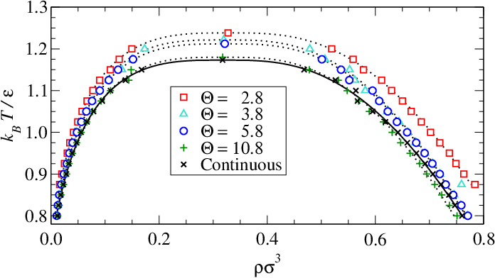
The simulation can reproduce the underlying model up to a specified energy approximation, i.e., $\left|E^{sim}-E^{model}\right|<\Delta E$.

Thomson, C., Lue, L. & Bannerman, MN. . 'Mapping continuous potentials to discrete forms'. J. Chem. Phys, 140, 034105 (2014)

These stepped approximations can closely reproduce the phase behavior of the LJ system:

Thomson, C., Lue, L. & Bannerman, MN. . 'Mapping continuous potentials to discrete forms'. J. Chem. Phys, 140, 034105 (2014)

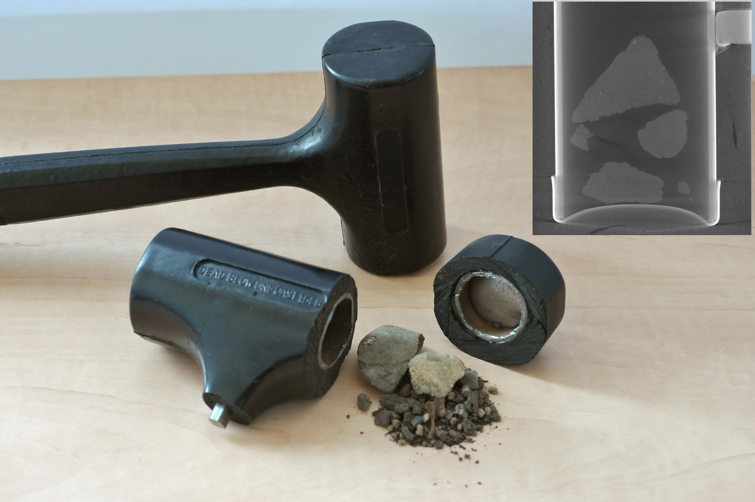
What about real granular systems?

M. Bannerman, J. E. Kollmer, A. Sack, M. Heckel, P. Müller, T. Pöschel, "Movers and shakers: Granular damping in microgravity," Phys. Rev. E, 84, 011301 (2011)

Experiment

Simulation

Comparison

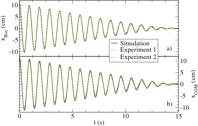
This led to the development of optimal design equations for dampers (see paper).