So far, we have discussed
single-effect
(single-stage) evaporators.
One of the problems of single-effect evaporators is that
they are energy intensive and require a lot of utilities.
Large quantities of steam are required to heat the
evaporator, and large amounts of cooling water are needed to
condense the output.
In process design, we utilise
heat integration
to maximise the efficiency of the process.
Heat integration can be used within a
multi-effect
(multi-stage) evaporator…
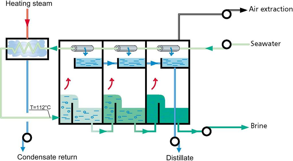
An example of heat integration, where energy recovered from
the condensers is used to preheat the feed stream in a
seawater desalination plant. The evaporation in each stage is
driven by pressure drops between the stages (note, this is not
a particularly efficient design!).
This form of
heat integration
is only available when the inlet stream is far from its boiling
point, as the
heat of condensation
is large when compared to the
sensible heat.
The pressure drops between stages must also be large to cause
significant boiling without additional heat input.
Both of these conditions are not often the case and they place a
constraint on the number of effects possible.
Let's consider the opposite system (inlet stream close to its
boiling point, heating in each stage).
There are two other forms of heat-integration in multi-effect
evaporators we can use…
In
forward-feed
multi-effect evaporators, the vapour from the first stage is
used to heat the liquid in the second stage.
Pressure drops are used between stages to change the boiling
point, and so generate a $\Delta T$ between the vapour and
liquid output from each stage.
The vapour and liquid streams from each stage flow
co-currently.
This configuration is used when the feed stream is already hot
(e.g., from a reactor), or if high temperatures must be avoided.
In
backward-feed
multi-effect evaporators, the liquid stream flows
counter-current
to the vapour streams.
Again, there is a pressure gradient between stages to facilitate
heat transfer, and so pumps are required between stages.
The advantages are that not all of the feed fluid needs to be
heated to the high boiling temperatures of the high-pressure
stage.
If the product is viscous, the concentrated (high-viscosity)
liquid is present at the highest temperature, thus reducing the
viscosity.
The barometric leg is a pipe with a column of water in it. The
weight of this water column drops the pressure in the final
stage, very cheap vacuum!
When choosing the number of stages, a trade-off between the
capital cost
and
running cost
determines the number of stages.
But, if we assume all streams are water/steam and a constant
latent heat of vaporisation, for each kilogram of steam, three
kilograms of feed are evaporated in the above diagram (steam economy${}\approx3$).
This greatly increases the economy of the evaporators. For
example, in sugar-beet factories, eight effect evaporators are
not uncommon (steam economy${}\approx8$!).
Distillation columns are
multi-stage evaporators, driven by the condensation
of a counter-current vapour phase, so this idea will
come in useful later.
The only difference is that for distillation we need to use
vapour-liquid equilibrium data to predict the split of
components in the vapour/liquid stream of each stage.
Back to multi-stage evaporator design (for now) to better
understand the heat and mass balance.
Distillation column, displaying the trays/stages and the
counter-current flows of vapour and liquid.
When evaporators are designed, you are usually given/determine:
available steam pressure, final stage, feed stream
specification, final target liquid concentration, overall heat
transfer coefficient estimates, and physical properties.
Our system is designed once we know the areas $A_1$,
$A_2\ldots$. But we need temperatures and heat fluxes
($A_i=Q_i\,U_i^{-1}\,\Delta T_i^{-1}$) and this depends on the
heat balance, which depends on the mass balance, which depends
on the heat balance,…
This is a implicit set of equations, which is very common.
Computers and humans alike solve these the same way. Guess some
values, work through all equations to calculate these values
again and compare.
You can think of this problem as a cycle: solve the mass balance
then solve the energy balance. At first, we guess the heat
balance results that are needed in the mass balance, then use
the solved mass balance to carry out the heat balance and
compare.
“Shooting” methods like this start at one point in
the cycle (i.e. the feed stream mass balance) and "shoot" to try
to meet the end of the cycle (the solved energy
balance/evaporator areas).
The better our initial guesses of the heat balance, the closer
our shot will land to the target (and the less shots we need to
take). If we miss, we have to try again.
So what can we do to get good guesstimations of results from the
heat balance? Use physically realistic approximations!
Let us assume that for this initial estimate, we can neglect the
heat of solution, boiling point rise and other concentration
effects.
We also neglect sensible heat (to heat the feed stream to
boiling point, or carried in the liquid phase between stages).
These assumptions imply that the heat transferred from the
condensing steam in the first evaporator, is recovered in the
latent heat of the vapour stream. \begin{align*} Q_1\approx
Q_2\approx Q_3\approx Q_{effect} \end{align*}
If we assume the latent heats of vapourisation are constant
($h_{fg,steam}\approx h_{fg,1}\approx h_{fg,2}$), we can use
another approximation that the flow rates of the vapour phases
are equal. \begin{align*} V_1\approx V_2\approx V_3 \end{align*}
Above are all useful approximate expressions as we can
immediately gain an initial estimate of the flows (and therefore
concentrations) in each evaporator. We can also generate useful
approximate energy balance expressions from these equations…
If we assume the duty and area of each effect/stage is equal
(actually a deliberate design choice, as building several
exactly the same sized evaporators is economical), using the
heat transfer equation we have \begin{align*}
\frac{Q_{effect}}{A_{effect}}\approx U_1 \Delta T_1\approx
U_2 \Delta T_2 \approx U_3 \Delta T_3 \end{align*}
Thus, the temperature difference in each stage is inversely
proportional to the heat transfer coefficient (this differs
between stages as the fluid has high changes in
concentration/viscosity/etc.).
We can rearrange the above expression \begin{align*} \Delta T_i
&\approx \frac{Q_{effect}}{A_{effect}} \frac{1}{U_i} &
\frac{\sum_i\Delta T_i}{\sum_i1/U_i} &\approx
\frac{Q_{effect}}{A_{effect}} \end{align*} (we summed the LHS
equation over all stages to give the RHS equation)
Any temperature is obtained by substituting for
$Q_{effect}/A_{effect}\approx U_j T_j$, \begin{align*} \Delta
T_1 \approx \frac{1}{U_1}\frac{\sum_i\Delta T_i}{\sum_i1/U_i}
\end{align*}
These expressions are useful as estimates for $U$ are available
(from experience), and the overal temperature difference is
defined from the steam and outlet temperatures
$\sum_i\Delta{}T_i=T_{3}-T_{steam}$.
To reiterate, in commercially available multi-effect evaporators
the heat transfer areas of each stage are usually identical as
they like to stamp-out the same design. \begin{align*}
A_1=A_2=A_3=A_{effect} \end{align*} ( This expression is not
approximate, it is a design constraint)
This is the final constraint on the iterative calculations. Once
you converge to a single size for all evaporators, you may stop
iterating.
The previous expressions are useful in the initial estimation
step, before attempting to converge on a solution for the
evaporator sizing.
We can make some additional educational assumptions to
demonstrate the relationship between single and multi-stage
evaporators…
If we assume the heat transfer coefficients are, on average, the
same \begin{align*} U_1\approx U_2\approx U_3\approx U_{effect}
\end{align*} Then the total heat transferred is \begin{align*}
Q_{total} &= Q_1+Q_2+Q_3\approx U_{effect} A_{effect}\sum_i
\Delta T_i\\ Q_{total} &\approx
U_{effect} A_{effect}\left(T_3-T_{steam}\right) \end{align*}
Thus, we can see that the multi-stage evaporator is equivalent
to a single stage evaporator with the same area, overall
temperature difference and average heat transfer coefficient.
However, the steam economy is significantly higher (we get much
more vapour, $V_{total} \neq Q_{total} / h_{fg}$).
We add to these approximate equations the exact mass balance
equations, around the whole multi-stage evaporator and around
each individual stage. \begin{align*} F &= V_1+V_2+V_3+L_3
& x_F F &= x_3 L_3\\ L_i&= V_{i+1} + L_{i+1} &
x_i L_i&= x_{i+1} L_{i+1} \end{align*}
We also have the corresponding energy balance equations.
In summary, assuming we have three stages/effects…