This article discusses some simple optimizations that can be made to accelerate GPU ray-traced volume renderings. These features are implemented in the upcoming version of DynamO/Coil to visualize hydrodynamic fields.
Volume rendering is a technique used to visualize volumes of data. This technique is very popular in Computational Fluid Dynamics (CFD) to aid researchers to look inside the system and see how fields of data (such as the pressure or density) vary in three dimensions.
The technique is also very popular in medical applications where it is used to reconstruct MRI data, and technicians can peel away layers of skin and flesh (see right) and look inside a patient with a click of the mouse instead of a slice of the scapel.
This technique can be computationally expensive (its essentially ray-tracing), but thanks to programmable GPU's, realtime techniques are available for rendering this sort of data.
There are many resources on the web that describe various techniques:-
These resources are better than anything I can write, so I'll assume you looked at them or already know about volume rendering. I'll discuss some general tricks to accelerate ray tracing in these systems.
If you have a ray-traced volume renderer, the simplest method to accelerate volume rendering is to simpy increase the ray step size. By increasing the step size, each ray/pixel requires less calculations, less texture lookups (these are really expensive!), and the framerate increase can be dramatic.
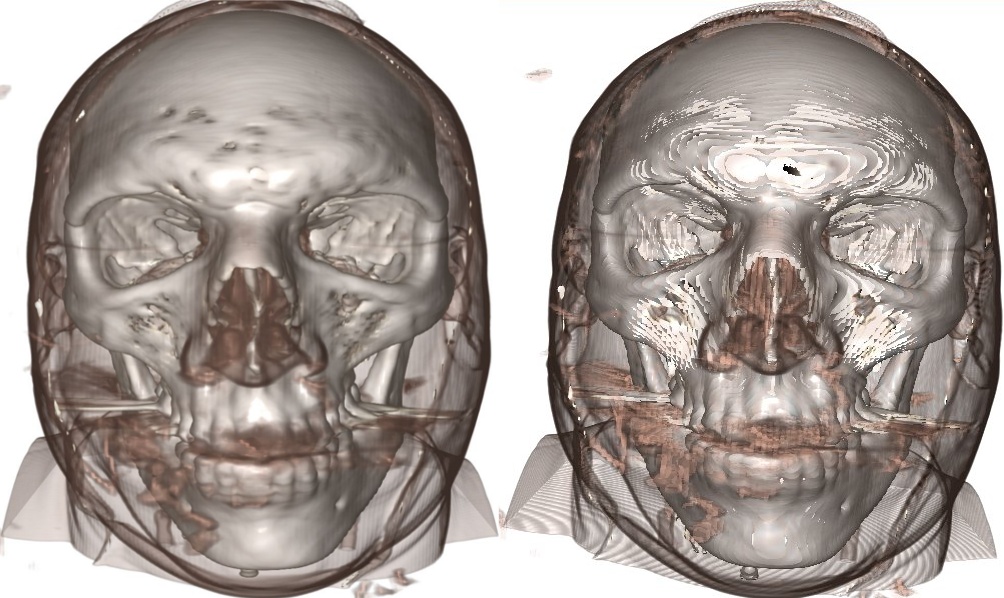
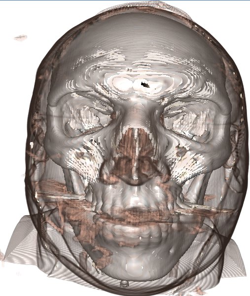
But a problem occurs when the ray step size approaches the size of a single Voxel, the image on the right shows what can happen.
The image has significant "banding" (see the circular patterns in the shoulders), and there are some bright white areas visible (around the forehead and cheeks).
At first this seems to be the cost of larger step sizes, but there are some tricks we can use to hide these effects. We'll deal with the white patches first....
The problem with the white patches is that the ray is outside a non-transparent region in one step and in the next it is deep within a dense region, it has skipped the surface.
To understand why this region is white, we have to understand how volume renderings are shaded (i.e., how the diffusive lighting works).
The reason why these rendering look so 3D is down to the diffusive lighting effect that has been applied. In computer graphics, this is usually calculated using Lambertian Reflection (see here for a full explanation) where the intensity \(I\) (brightness) at a pixel is proportional to the angle between the light source direction \({\bf {L}}\) and the surface normal \({\bf{}n}\)
\(I\propto{\bf{}n}\cdot{\bf{}L}\)
But how is the normal of a voxel defined? A surface has a well defined normal, but how do you turn voxels into surfaces? To get around this, the gradient of the density is used to define an "effective" surface normal.
\({\bf{}n}(x,y,z)\approx\textrm{normalize}\left(\nabla\rho(x,y,z)\right)\)
Here,\(\rho(x,y,z)\) is the density at our Voxel and \(\nabla\) is the gradient operator. Typically, the gradient is approximated using the central difference approximation
\(\nabla_x\rho(x,y,z)\approx\frac{\rho(x+1,y,z)-\rho(x-1,y,z)}{2}\)
This equation is repeated for each dimension x,y,z, and these three components are the components of the surface normal.
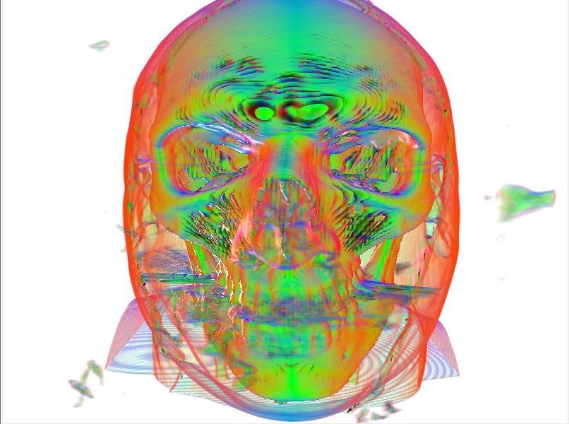
So we have defined an effective surface normal, why are those voxels white? Well, the ray has jumped into a high density region (the skull). And inside the skull (for this dataset) all the voxels have exactly the same value of density! This is because the scanner (or whatever took the image) has run out of range to describe the data and just set the density to the max value (255 in this 8bit data). But, if a voxel is surrounded by other voxels all with the same density, this means that the gradient is zero!
\(\nabla\rho(x,y,z)={\bf{}0}\)
We can't make a normal out of this as a zero vector has no direction. So instead, no shading is applied here and we either get bright white or dark black spots instead, depending on the shaders implementation.
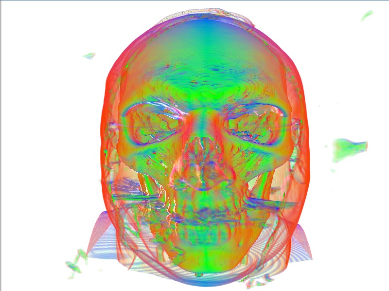
We can visualize this if we render the normal information as a color. We can see that the white areas in the above picture correspond to areas without gradients (black areas in right image).
One typical solution to this problem is to blur the components of the gradient.
The gradients are calculated as usual, but a gaussian blur is used afterwards to spread and smudge the surface normals from the surface voxels into the voxels without a gradient. This way, voxels without a gradient will still get some surface-normal information from nearby voxels with the added benefit that the rendering as a whole becomes a little smoother.
The problem with this technique is that blurring normals is not really well defined and it is hugely expensive! If you wish to render live data with this technique, all of your time will be spent on the 3D gaussian filter pass.
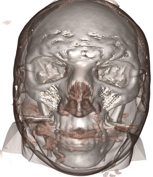
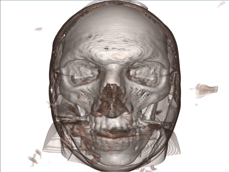
This technique still doesn't cure all the problems though, a 5x5 gaussian filter was applied to the normal data and the result is presented on the left.
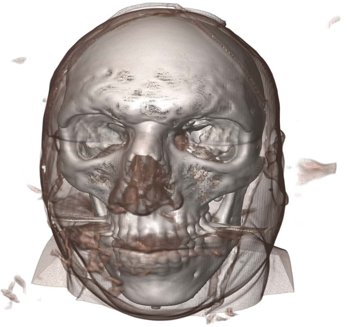
Instead of blurring we can use another trick at draw time, inside the fragment/pixel shader. While our ray is stepping through the volume, we keep track of the previous step's normal. If the ray enters a region where there are no well defined normals, the ray simply reuses the old normal!
This technique works very well as even though the area outside the solid area is transparent, it still usually contains a density gradient, and this gradient is close to what the true gradient of the surface is. We also only look at the gradient which is relevant to the side of the surface we're on!
We can compare the benefits of this technique below (click for high resolution), before we enable normal reuse we have
And after we have
A great improvement, still some artifacts but very cheaply rendered!
The final artifact we will fix is the banding present in all the above images. This banding is also known as "aliasing", and is due to the large step size missing small changes in the image.
A common technique to remove aliasing is known as dithering. The trick is to introduce just enough randomness in the image to remove the aliases and replace them with speckles. This random noise must be high frequency and repeatable (i.e., the image shouldn't flicker).
This is remarkably simple to implement in GLSL, to the starting point of every ray, a random fraction of the step size should be added. The following GLSL does this using the fragment coordinate as a seed.
To finish we'll do a before and after dithering (again, you can click on the images for a higher resolution version)....
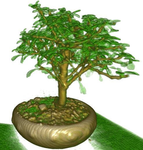
Finally, the image at the top of this article was rendered with a smaller step size to clearly resolve the small holes in the volume around the cheek and forehead.
The current version of my Volume rendering shaders is available here: volumeShader.hpp
The volume data of a male skull and bonsai tree was obtained from this website and I'd like to thank Kyle Hayward and Philip Rideout for their excellent tutorials on volume ray tracing.