Applications of Energy Balances
Review
- In the previous lecture, we derived the general energy balance equation. \begin{align*} \rho\frac{\partial e}{\partial t} &= - \rho v_i \nabla_i e - \nabla_i q_i - \nabla_i(\tau_{ij} v_j) - \nabla_i(p v_i) + \sigma_{energy} \end{align*}
- We defined the Laplace operator $\nabla^2$, and noted its special definitions in different coordinate systems!
-
We also defined Fourier's law of conduction: \begin{align*} \boldsymbol{q} = -k \nabla T \end{align*} and noted it's definitions in different coordinate systems (see right).
Rectangular Cylindrical Spherical $q_x = -k\frac{\partial T}{\partial x}$ $q_r = -k\frac{\partial T}{\partial r}$ $q_r = -k\frac{\partial T}{\partial r}$ $q_y = -k\frac{\partial T}{\partial y}$ $q_\theta = -k\frac{1}{r}\frac{\partial T}{\partial \theta}$ $q_\theta = -k\frac{1}{r}\frac{\partial T}{\partial \theta}$ $q_z = -k\frac{\partial T}{\partial z}$ $q_z = -k\frac{\partial T}{\partial z}$ $q_\phi = -k\frac{1}{r \sin\theta}\frac{\partial T}{\partial \phi}$ Fourier's Law in all coordinate systems - We will now take a look at using these equations in heat transfer, just like we did for flow problems and the Cauchy momentum equation.
Simplifying the Energy Balance by removing the Cauchy equation
- Before we continue, we will simplify the energy balance equation a bit more. \begin{align*} \rho\frac{\partial e}{\partial t} &= - \rho v_i \nabla_i e - \nabla_i q_i - \nabla_i(\tau_{ij} v_j) - \nabla_i(p v_i) + \sigma_{energy} \end{align*}
- When we derived the momentum equation, we factored and cancelled a term involving the continuity equation.
- In getting to the above energy equation, we also factored out the continuity equation.
- But we can also factor out the momentum equation from the energy equation.
- Take the momentum equation… \begin{align*} \rho\frac{\partial v_i}{\partial t} &= -\rho v_j \nabla_j v_i - \nabla_j \tau_{ji} - \nabla_i p + \rho g_i \end{align*}
- Multiply it by $v_i$ (this is equivalent to dotting $\boldsymbol{v}\cdot{}$ to all terms) \begin{align*} \rho v_i\frac{\partial v_i}{\partial t} &= -\rho v_j v_i \nabla_j v_i - v_i \nabla_j \tau_{ji} - v_i \nabla_i p + \rho v_i g_i\\ \frac{1}{2}\rho\frac{\partial v_i v_i}{\partial t} &= -\rho v_j \nabla_j \frac{v_i v_i}{2} - v_i \nabla_j \tau_{ji} - v_i \nabla_i p + \rho v_i g_i \end{align*}
- Next we insert the definition of the energy $e=\frac{1}{2}v^2 + \cancelto{e_{pot.}(\boldsymbol{r})}{0} + U$ into the energy balance, ignore gravity (and thus the only potential term we know) and subtract the above equation \begin{align*} \rho\frac{\partial e}{\partial t} &= - \rho v_i \nabla_i e - \nabla_i q_i - \nabla_i(\tau_{ij} v_j) - \nabla_i(p v_i) + \sigma_{energy} \\ \rho\frac{\partial U}{\partial t} =& -\rho v_i \nabla_i U - \nabla_i q_i - \tau_{ji} \nabla_j v_i - p \nabla_i v_i +\sigma_{energy} \end{align*}
- This is as far as we can go while remaining “exact” (we ignored gravity, but we've ignored many forms of energy).
- However, there is a useful assumption if we are in a liquid or solid, the internal energy has little or no pressure dependence \begin{align*} {\rm d}U = C_p {\rm d}T + \cancelto{0}{\left(\frac{\partial U}{\partial p}\right)_T {\rm d} P} \end{align*}
- And we have another form of the energy balance \begin{align*} \rho C_p\frac{\partial T}{\partial t} =& -\rho C_p v_j \nabla_j T - \nabla_i q_i - \tau_{ji} \nabla_j v_i - p \nabla_i v_i +\sigma_{energy} \end{align*}
- This form easily reduces to the heat equation for solids/stationary liquids ($\boldsymbol{v}=\boldsymbol{0}$ ). \begin{align*} \rho C_p\frac{\partial T}{\partial t} =& - \nabla_i q_i +\sigma_{energy} \end{align*}
Example: Conduction in an Electrically Heated Wire
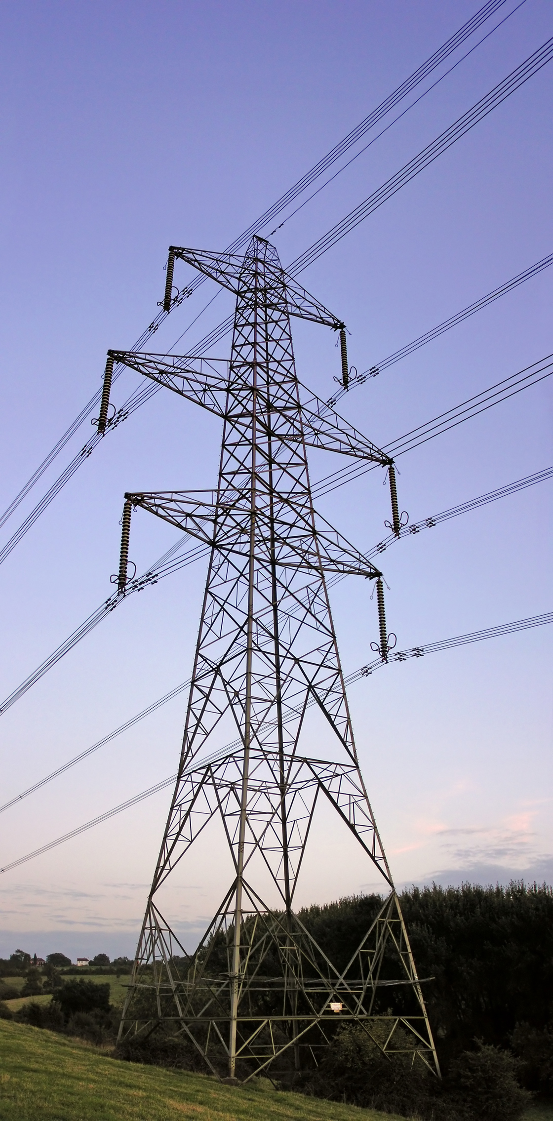
- Let's take a look at the dissipation of heat in a wire on an electricity pylon.
- The transmission of an electric current is an irreversible process, and some electrical energy is converted into heat.
- Joule determined that the amount of heat energy produced per unit volume is given by \begin{align*} \sigma_{energy}^{current} = \frac{I^2}{k_e} \end{align*} where $I$ is the current density and $k_e$ is the electrical conductivity of the transmission material.
- We will use this as an expression for the rate of heat generation in a wire (we do not track electrical energy in our energy balance equation, just heat, so this term is a heat energy “generation” term).
- Taking our general balance equation, we have \begin{align*} \rho C_p\frac{\partial T}{\partial t} =& -\rho C_p \boldsymbol{v} \cdot\nabla T - \nabla\cdot\boldsymbol{q} - \boldsymbol{\tau}:\nabla\boldsymbol{v} - p \nabla\cdot\boldsymbol{v} +\frac{I^2}{k_e} \end{align*} (Note, $\boldsymbol{\tau}:\nabla\boldsymbol{v}=\tau_{ij}\nabla_iv_j$ for Cartesian coordinates)
- We note that wires are usually made out of solid material (aluminium), so we can state that $\boldsymbol{v}=0$ , and cancel all terms with the velocity in them: \begin{align*} \rho C_p\frac{\partial T}{\partial t} =& - \nabla\cdot\boldsymbol{q} +\frac{I^2}{k_e} \end{align*}
- Assuming the system is at steady state (no severe weather changes or sudden surges in electricity demand), we have \begin{align*} \nabla\cdot\boldsymbol{q} =\frac{I^2}{k_e} \end{align*}
\begin{align*} \nabla\cdot\boldsymbol{q} =\frac{I^2}{k_e}
\end{align*}
- Assuming our wires are cylinders, we should use cylindrical coordinates.
- Our expression becomes \begin{align*} \nabla\cdot\boldsymbol{q}=\frac{1}{r}\frac{\partial}{\partial r}\left(r q_r\right) + \frac{1}{r}\frac{\partial q_\theta}{\partial \theta}+ \frac{\partial q_z}{\partial z}= \frac{I^2}{k_e} \end{align*}
- To simplify this problem, we assume that the wire is cooled evenly by the wind so that there is no variance in external temperature with the angle $\theta$ or position on the wire $z$ .
- This makes the problem symmetric in $z$ and $\theta$ .
\begin{align*} \frac{1}{r}\frac{\partial}{\partial r}\left(r
q_r\right) + \frac{1}{r}\frac{\partial q_\theta}{\partial
\theta}+ \frac{\partial q_z}{\partial z}= \frac{I^2}{k_e}
\end{align*}
- Whenever there is symmetry, there is no transport.
- This is because there are no gradients or flow across a symmetry as the values of all functions are equal either side of the symmetry.
- All transport is driven by gradients (convective, Newton's Law, Fourier's Law, and Fick's First Law).
- Our problem is rotationally symmetric in $\theta$ and has translational invariance/symmetry in $z$ so $q_\theta=q_z=0$ and we have \begin{align*} \frac{1}{r}\frac{\partial}{\partial r}\left(r q_r\right) = \frac{I^2}{k_e} \end{align*}
\begin{align*} \frac{1}{r}\frac{\partial r q_r}{\partial
r}=\frac{I^2}{k_e} \end{align*}
- Integrating this expression, we have \begin{align*} q_r=\frac{I^2}{k_e}\left(\frac{r}{2} + \frac{C}{r}\right) \end{align*}
- Hopefully you have a feeling of deja vu as you note that in the centre of the wire where $r=0$ , the heat flux cannot reach infinity so we must have $C=0$ .
- We could also note that at $r=0$ we are on an axis of symmetry and so $q_r=0$ , also requiring $C=0$ .
- Our final expression for the heat flux is then: \begin{align*} q_r=\frac{I^2}{2 k_e}r \end{align*}
-
Now let's use the definition of Fourier's law in 3D
Rectangular Cylindrical Spherical $q_x = -k\frac{\partial T}{\partial x}$ $q_r = -k\frac{\partial T}{\partial r}$ $q_r = -k\frac{\partial T}{\partial r}$ $q_y = -k\frac{\partial T}{\partial y}$ $q_\theta = -k\frac{1}{r}\frac{\partial T}{\partial \theta}$ $q_\theta = -k\frac{1}{r}\frac{\partial T}{\partial \theta}$ $q_z = -k\frac{\partial T}{\partial z}$ $q_z = -k\frac{\partial T}{\partial z}$ $q_\phi = -k\frac{1}{r \sin\theta}\frac{\partial T}{\partial \phi}$ Fourier's Law in all coordinate systems - Selecting the correct definition, we have \begin{align*} \frac{\partial T}{\partial r} = -\frac{I^2}{2 k_e k}r \end{align*}
\begin{align*} q_r&=\frac{I^2}{2 k_e}r\\ \frac{\partial
T}{\partial r} &= -\frac{I^2}{2 k_e k}r\\ \end{align*}
- Assuming $k$ is constant (it actually depends on the temperature), we can integrate this expression to gives us the temperature profile. \begin{align*} T &= \frac{I^2}{4 k_e k}\left(C-r^2\right) \end{align*}
- For now, we will use the simple boundary condition that the exterior of the wire ($r=R$ ) is held at a fixed temperature $T=T_0$ to solve for the constant $C$ to give \begin{align*} T - T_0 &= \frac{I^2 R^2}{4 k_e k}\left(1-\frac{r^2}{R^2}\right) \end{align*}
\begin{align*} q_r&=\frac{I^2}{2 k_e}r\\ T - T_0 &=
\frac{I^2 R^2}{4 k_e k}\left(1-\frac{r^2}{R^2}\right)
\end{align*}
- A final derivation is to find the total heat flux at the surface of the wire $Q_r|_{wall}$ .
- Setting $r=R$ in the equation for the heat flux $q_r$ and multiplying by the surface area of the wire gives us \begin{align*} Q_r|_{wall} = \frac{\pi R^2 L I^2}{k_e} \end{align*}
- This could also be immediately derived by noting that at steady state, all heat generated in the wire must flow out.
\begin{align*} q_r&=\frac{I^2}{2 k_e}r\\ T - T_0 &=
\frac{I^2 R^2}{4 k_e k}\left(1-\frac{r^2}{R^2}\right)\\
q_r|_{wall} &= \frac{\pi R^2 L I^2}{k_e} \end{align*}
- Our solution is mathematically identical to the solution for momentum transport in pipes! \begin{align*} \tau_{rz} &= \frac{\Delta p}{2 L}r & v_z &= -\frac{\Delta p R^2}{4 \mu L}\left(1 - \frac{r^2}{R^2}\right)\\ \tau_{rz}|_{wall} &= \Delta p \pi R^2 \end{align*}
- We have found an analogous process for flow profiles in heat transfer! This is the power of combined Momentum, Heat, and Mass transfer studies.
- With a bit of thought you should be able to immediately write down the expression for electrical heating in a tubular conductor (think flow in an annulus).
Real systems
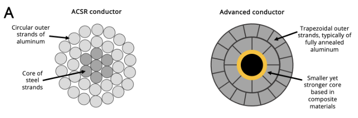
- An annulus is closer to the real case for wires used in modern electricity pylons!
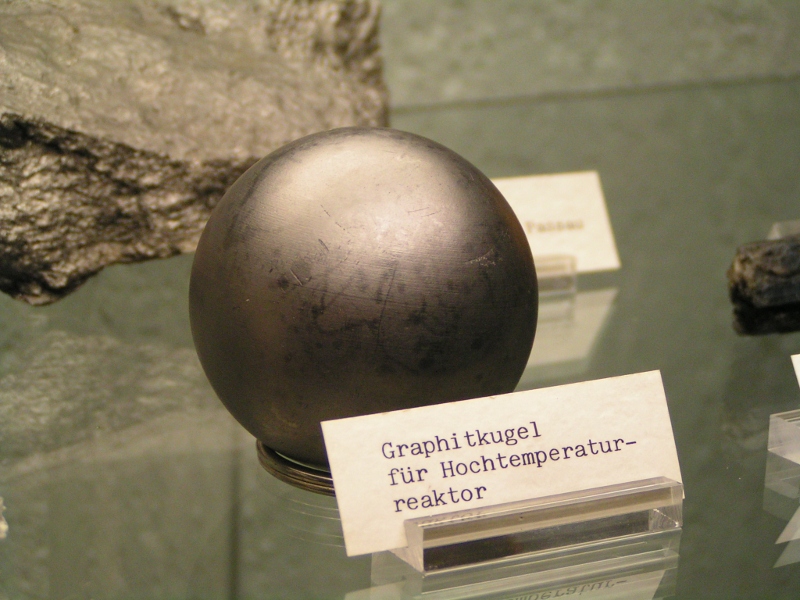
Example: Spherical Nuclear Fuel
- Let's take another look at a heat transfer problem.
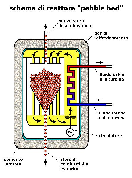
- There is an unusual design of nuclear reactor called a pebble bed reactor .
- Each pebble consists of a sphere of fissionable material with a radius $R^{(F)}$ surrounded by a spherical shell of graphite “cladding” to a radius $R^{(C)}$ .
- Due to the nature of nuclear fission, the rate of heat generation is not uniform within the sphere, it depends on temperature and the production of neutrons within the sphere.
- As a first approximation, it is assumed that the generation rate is given by \begin{align*} \sigma_{energy}^{fission} = \sigma_0 \left(1+b\left(\frac{r}{R^{(F)}}\right)^2\right) \end{align*}
- Taking our general balance equation, we have \begin{align*} \rho C_p\frac{\partial T}{\partial t} =& -\rho C_p \boldsymbol{v} \cdot\nabla T - \nabla\cdot\boldsymbol{q} - \boldsymbol{\tau}:\nabla\boldsymbol{v} - p \nabla\cdot\boldsymbol{v} +\sigma_{energy} \end{align*}
- Again, the system is solid so we can state that $\boldsymbol{v}=0$ . \begin{align*} \rho C_p\frac{\partial T}{\partial t} =&- \nabla\cdot\boldsymbol{q} +\sigma_{energy} \end{align*}
- Assuming that the nuclear reactor is at steady state, we have \begin{align*} \nabla\cdot\boldsymbol{q} =\sigma_{energy} \end{align*}
- Choosing spherical coordinates, we assume due to symmetry that only the radial flux is important ($q_\theta=q_\phi=0$), and we have \begin{align*} \frac{1}{r^2}\frac{\partial}{\partial r}\left(r^2 q_r\right) + \frac{1}{r\sin\theta}\frac{\partial}{\partial \theta}\left(\cancelto{0}{q_\theta}\sin\theta\right)+ \frac{1}{r\sin\theta}\frac{\partial \cancelto{0}{q_\phi}}{\partial \phi} =\sigma_{energy} \end{align*}
\begin{align*} \frac{1}{r^2}\frac{\partial}{\partial
r}\left(r^2 q_r\right)=\sigma_{energy} \end{align*}
- We actually have two coupled equations to solve, one for the core of fissionable material (where there is heat production): \begin{align*} \frac{1}{r^2}\frac{\partial}{\partial r}\left(r^2 q_r^{(F)}\right) &= \sigma_0 \left(1+b\left(\frac{r}{R^{(F)}}\right)^2\right) \end{align*}
- And one for the aluminium cladding (where there is no heat production): \begin{align*} \frac{1}{r^2}\frac{\partial}{\partial r}\left(r^2 q_r^{(C)}\right) &= 0 \end{align*}
\begin{align*} \frac{1}{r^2}\frac{\partial}{\partial
r}\left(r^2 q_r^{(F)}\right) &= \sigma_0
\left(1+b\left(\frac{r}{R^{(F)}}\right)^2\right) \\
\frac{1}{r^2}\frac{\partial}{\partial r}\left(r^2
q_r^{(C)}\right) &= 0 \end{align*}
- Our equations then become \begin{align*} \frac{\partial}{\partial r}r^2 q^{(F)}_r &= \sigma_0 r^2 \left(1+b\left(\frac{r}{R^{(F)}}\right)^2\right) \\ \frac{\partial}{\partial r}r^2 q^{(C)}_r &= 0 \end{align*}
\begin{align*} \frac{\partial}{\partial r}r^2 q^{(F)}_r &=
\sigma_0 r^2 \left(1+b\left(\frac{r}{R^{(F)}}\right)^2\right)\\
\frac{\partial}{\partial r}r^2 q^{(C)}_r &= 0 \end{align*}
- We can integrate these equations to give \begin{align*} q^{(F)}_r &= \sigma_0\left(\frac{r}{3}+\frac{b r^3}{5 \left(R^{(F)}\right)^2}\right) + \frac{C_1^{(F)}}{r^2}\\ q^{(C)}_r &= \frac{C_1^{(C)}}{r^2} \end{align*}
- At $r=0$ we know that the flux in the fissionable material must be finite so $C_1^{(F)}=0$ . In fact, as the problem is symmetric at the origin, we know the flux is zero in the centre.
\begin{align*} q^{(F)}_r &=
\sigma_0\left(\frac{r}{3}+\frac{b r^3}{5 \left(R^{(F)}\right)^2}\right)\\
q^{(C)}_r &= \frac{C_1^{(C)}}{r^2} \end{align*}
- We know that both heat fluxes at $r=R^{(F)}$ must equal $q_r^{(F)}=q_r^{(C)}$ , so we can determine $C_1^{(C)}$ to give. \begin{align*} q^{(C)}_r &= \frac{\sigma_0 \left(R^{(F)}\right)^3}{r^2}\left(\frac{1}{3}+\frac{b}{5}\right) \end{align*}
\begin{align*} q^{(F)}_r &=
\sigma_0\left(\frac{r}{3}+\frac{b r^3}{5 \left(R^{(F)}\right)^2}\right)\\
q^{(C)}_r &=
\frac{\sigma_0 \left(R^{(F)}\right)^3}{r^2}\left(\frac{1}{3}+\frac{b}{5}\right)
\end{align*}
-
Again, we must check the definition of Fourier's law in
Spherical coordinates.
Rectangular Cylindrical Spherical $q_x = -k\frac{\partial T}{\partial x}$ $q_r = -k\frac{\partial T}{\partial r}$ $q_r = -k\frac{\partial T}{\partial r}$ $q_y = -k\frac{\partial T}{\partial y}$ $q_\theta = -k\frac{1}{r}\frac{\partial T}{\partial \theta}$ $q_\theta = -k\frac{1}{r}\frac{\partial T}{\partial \theta}$ $q_z = -k\frac{\partial T}{\partial z}$ $q_z = -k\frac{\partial T}{\partial z}$ $q_\phi = -k\frac{1}{r \sin\theta}\frac{\partial T}{\partial \phi}$ Fourier's Law in all coordinate systems - We can then rewrite our problems in terms of the temperature profile.
\begin{align*} \frac{\partial T^{(F)}}{\partial r} &=
-\frac{\sigma_0}{k^{(F)}}\left(\frac{r}{3}+\frac{b r^3}{5 \left(R^{(F)}\right)^2}\right)\\
\frac{\partial T^{(C)}}{\partial r} &=
-\frac{\sigma_0 \left(R^{(F)}\right)^3}{k^{(C)} r^2}\left(\frac{1}{3}+\frac{b}{5}\right)
\end{align*}
- Again assuming constant thermal conductivity we can integrate these expressions.
- We then need boundary conditions for the constants, the first is that the temperatures are equal at the bonded interface \begin{align*} T^{(F)} &= T^{(C)} & \text{for} \quad r=R^{(F)} \end{align*}
- We will also assume the surface temperature of the particle is known \begin{align*} T^{(C)} &= T_0 & \text{for} \quad r=R^{(C)} \end{align*}
- The final expressions are enormous, for the fissionable material we have \begin{align*} T^{(F)} -T_0 & \\ =& \frac{\sigma_0 \left(R^{(F)}\right)^2}{3} \left\{\frac{1}{2 k^{(F)}}\left[1-\left(\frac{r}{R^{(F)}}\right)^2 + \frac{3}{10} b\left(1-\left(\frac{r}{R^{(F)}}\right)^4\right)\right]\right.\\ &\quad\left.+\frac{1}{k^{(C)}}\left(1+\frac{3 b}{5}\right)\left(1-\frac{R^{(F)}}{R^{(C)}}\right)\right\} \end{align*}
- For the cladding we have \begin{align*} T^{(C)} -T_0 = \frac{\sigma_0 \left(R^{(F)}\right)^2}{3 k^{(C)}} \left(1+\frac{3 b}{5}\right) \left(\frac{R^{(F)}}{r}-\frac{R^{(F)}}{R^{(C)}}\right) \end{align*}
- We can see the temperature increases towards the centre of each particle.
- Its vital that the temperature of the fissionable material is monitored as a design parameter!
Learning Objectives
- The general energy balance equation is: \begin{align*} \rho\frac{\partial U}{\partial t} &= -\rho v_j \nabla_j U - \nabla_i q_i - \tau_{ji} \nabla_j v_i - p \nabla_i v_i +\sigma_{energy} \end{align*}
- A simpler heat balance equation is derived using the assumption that the internal energy has only a weak pressure dependence: \begin{align*} \rho C_p\frac{\partial T}{\partial t} &= -\rho C_p v_j \nabla_j T - \nabla_i q_i - \tau_{ji} \nabla_j v_i - p \nabla_i v_i +\sigma_{energy} \end{align*}
- We have solved our first conduction problem for heat transfer in an electrically heated wire and found it is analogous to velocity profiles in a pipe.
- We solved for the temperature profile in a nuclear fuel pellet (our first spherical coordinate problem).
- This all required being careful with terms involving $\nabla$ terms.
- But our boundary conditions for the systems were unsatisfactory, all systems had fixed temperatures at the surface but this is not realistic…
- … we need to set other boundary conditions on heat transfer problems.